Seminar on multivariate data analysis of secondary ion mass spectrometry given by Dr Gustavo F Trindade as part of the “SIMS workshop” series organised at the University of Nottingham
Multivariate analysis of mass spectrometry imaging data | contact@mvatools.com
Seminar on multivariate data analysis of secondary ion mass spectrometry given by Dr Gustavo F Trindade as part of the “SIMS workshop” series organised at the University of Nottingham
Presented by Dr Gustavo F Trindade as part of the “SIMS Workshops” series organised at the University of Nottingham

Presented by Dr Gustavo F Trindade as part of the “SIMS Workshops series” organised at the University of Nottingham.
Presented by Dr Gustavo F Trindade as part of the “SIMS workshops” series organised at the University of Nottingham.

Presented by Dr Gustavo F Trindade as part of the “SIMS Workshop” series organised at the University of Nottingham

Dear simsMVA user
This is just a quick guide on how to set up and run the MATLAB version of simsMVA.
1 – unzip the files
2- inside MATLAB, find the folder, right-click on it and select “add to path -> selected folder”

3 – go to the command window and type in “simsMVA”
You will need to do step 2 every time you restart MATLAB, but once the folder is in the search path, you can run multiple instances of simsMVA
If you want to permanently add the folder to your search path, you can go to MATLAB’s “Home” tab and click on “Set path” (This will require admin rights)


For this tutorial you will be using the example data “Adhesive” from the examples menu in simsMVA. The data consists of secondary ion maps of the surface of a packaging adhesive. The aim is to produce the following figure:

Where the left-hand side contains an overlay of three NMF components intensities and the right-hand side contains their characteristic spectra.
To load the example dataset, click on “Examples” on the top menu and select “Imaging (Adhesive)”, then click on the new tab created.

Pre-process the data by normalising all maps by total ion counts and Poisson-scaling. Choose a more appropriate colour map that would help to identify whether everything is OK with the pre-processed data.
For this example, NMF was performed in a subset of only 3% of the pixels. This is done by selecting “Sample 3%” in the subsampling drop-down menu, then click the “NMF” ![]() button and set the input parameters:
button and set the input parameters:
A new tab is then created with the NMF results. Click on it.
Now we have the data needed for the overlay. To produce it, click the “Overlay” button on the “Components” panel. If you intend to print it or include it in a white-background slide, change simsMVA colour scheme by clicking “Theme” on the top menu bar and selecting a white background theme such as “Almond Milk”.
The “Overlay” window consists of three panels: “Control”, “Overlay” and “Components”. On the “Control” panel, the “Add” buttons allow you to add individual components to the overlay and the coloured button next to it sets their respective colours. For this image, a base colourmap (“hsv”), without much tweaking, was enough to produce good results. In cases where there are more than three components, you may want to tweak the colours of a base colourmap in order to enhance contrast.

Note that the plots on the right-hand side are connected, so if you use the magnifying lens ![]() to zoom in any of the plots, all three plots will show the same x-scale.
to zoom in any of the plots, all three plots will show the same x-scale.

Once you are happy with the colour and sizes, you can export the figure by clicking “File->Export setup…”, select appropriate rendering and export it to your desired compression format.

A bit of background
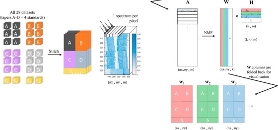
Non-negative matrix factorisation (NMF)1,2 is a non-supervised machine learning method that seeks to reduce the dimensionality of a dataset down to a few “pure” components. For the application of NMF to ToF-SIMS images, the data is unfolded into a Matrix A containing samples (pixels) in rows and variables (spectral channels) in columns. The method then finds an approximate factorisation A ≈ WH into non-negative factors W and H. H is interpreted as the characteristic spectra of components and W is interpreted as the “concentration” distribution of the components over the samples. The number of components is defined by the inner dimension of the product WH, as shown in the figure below:

