The simsMVA app is developed on Matlab 2016b and, alongside with in-house developed functions, makes use of the Statistics and Machine Learning and the Image Processing toolboxes. The main window will contain a menu bar with three options: “New tab”, “Theme” and “Help”. The “New tab” menu contains four different options: “Spectra”, “Images”, “Profiles” and “3D”. Every time one of these options are selected, a new tab is created under a name that the user is prompted to give. The “Theme” menu contains a set of different colour schemes that can be applied to the GUI. A detailed description of each feature present in each kind of tab is given in Table 1.
A Spectra tab is shown in Figure 5. It contains a java-based table (Copyright (c) 2015, Yair Altman. All rights reserved) with all loaded data: peak areas of different samples and their associated mass and labels. The first column contains tick boxes that allow the user to unselect specific variables prior to multivariate analysis. The figures on the left hand side show a plot of the average peak list for all samples. The upper image will always show the original data and the bottom figure will show the pre-processed data. The figure on the bottom left will contain a scatter plot where the user can select which peak areas to plot against each other. A Profiles tab is shown Figure 6. It contains a table on the right hand side that allows the selection of which peak intensity profile to plot on the set of axis on the left hand side. An Images tab is shown in Figure 7. The image on the top left hand side will show the intensity maps for the selected ion. The two plots on the right hand side will show the intensity distribution of the peak list (after selected pre-processing) outside (top) and inside (bottom) of the region of interest determined by a red polygon on the left hand side map. The image on the bottom left will contain an RGB overlay of three different mass fragments maps selected by the user. A 3D tab is shown in Figure 8. The image on the top left side will show the intensity maps for the selected ion at the selected level. The two plots on the right hand side will show the intensity distribution of the peak list (after selected pre-processing) outside (top) and inside (bottom) of the region of interest determined by a red polygon on the left hand side map. The image on the bottom left will have a 3D map of intensities with a slice on the currently selected level.
Both images and 3D tabs will have the option of subsampling the data using low discrepancy which have been shown to generate, in much less time, results as good as if the whole dataset was processed [13–15].
Table 1: Detailed description of each feature present in each kind of tab.
| Item | Description | Spectra | Images | Profiles | 3D |
| New list (Load)
|
Opens a file selection dialog that allows the user to select one or more .txt (Spectra and Profiles) or .BIF6 (Images and 3D) files exported from the SurfaceLab software. Files for different set of samples must have the same peak list. | X | X | X | X |
| Add extra
|
Opens a file dialog that allows the user to select one or more .txt files exported from the SurfaceLab software that will be added to the already loaded files. | X | |||
| Set groups
|
Pops up a window with all sample names. The user can then give the same name to technical repeats and select which samples to be considered for analysis. One the groups are set, the scatter plot on the bottom left figure will be updated with matching colours for samples within the same group. | X | |||
| PCA
|
Performs principal components analysis and creates an “MVA results” tab with the PCA results. | X | X | X | X |
| NMF
|
Pops up a window (NMF menu) that allows the user to select input parameters for non-negative matrix factorisation (Algorithm, number of components, number of iterations). The Run creates an “MVA results” tab with the NMF results. | X | X | X | X |
| PLS
|
Under construction | X | |||
| k-means
|
Pops up a window (K-means menu) that allows the user to select input parameters of the Matlab kmeans function (Distance, number of clusters, number of iterations and number of replicates). The Run button creates an “MVA results” tab with the k-means clustering results. | X | X | ||
| Plot intensities | Pops up a window similar to a Scores viewer that allow the user to plot intensities of individual mass peaks for all samples. | X | |||
| Mass filter | Pops up a menu that allows the user to filter out inorganic or organic mass fragments prior to multivariate analysis. | X | |||
| Set mass range/Mass ROI | Changes the mouse cursor to a cross. The user then has to click on two points on the top left hand side figure to select the mass range within the peak list in which the analysis will be done. The selected masses will be shown in red colour. | X | X | X | |
| Pre-processing | Drop down menu with different data pre-processing options. | X | X | X | X |
| Bootstrap resampling | Resamples the data within individual groups based on their multivariate distribution (requires more than 3 samples in the same “group”). | X | |||
| Save project
|
Opens a save file dialog that allows the user to save the project as a .mat file. | X | |||
| Load project
|
Opens a load file dialog that allows the user to open any saved projects. | X | |||
| Make report | Generates a PCA results report in a .doc file. | X | |||
| Mass selector | Drop down menu to select, within the exported peak list, which ion map to display. The images will automatically be updated upon selection. | X | X | ||
| Normalise | Drop down menu to select one ion map to be used as a normalisation factor for all other maps. | X | X | ||
| Binning | Drop-down menu for resizing the dataset by binning down the number of pixels. The higher the binning level is, the smaller the images are. | X | X | ||
| Smoothing | Drop-down menu for smoothing the dataset pixel-wise (images and 3D) or level-wise (Profiles). It applies a Gaussian kernel filter to all ion maps. | X | X | X | |
| Colourmap | Drop-down menu to switch amongst Matlab standard colour maps for displaying the ion maps. | X | X | ||
| Whole image/Use ROI | Selector to determine whether to perform MVA in all pixels/voxels or in a low discrepancy subset of samples ranging from 1% to 50% of the total or a user determined region-of-interest (ROI) determined by a red polygon in the right hand side figure. | X | X | ||
| Save figure (change to save data/project) | Opens a file save dialog that enables the user to save all displayed figures (without buttons and menus) in a .png file. | X | X | X | |
| Line scan
|
Changes the mouse cursor to a cross. The user then has to click on two or more points on the right hand side map and press enter to display (in the figure at the bottom left hand side) the ion intensity across the line connecting the selected points. | X | X | ||
| Overlay
|
Pops up a window with three mass selectors that will one different ion maps per channel in a RGB image displayed under the selectors. | X | X | ||
| Log scale | Toggle button to switch the plot y-scale between linear and log. | X | |||
| Normalisation | Normalise all profiles data by either their maximum value or the sum of all profiles. | X | |||
| Select all | (Button is missing. Fix it) | X | |||
| Level selector | Drop down menu to select which level of the 3D data to display. | X | |||
| Normalise by | Drop down menu to select one ion map to be used as a normalisation factor for all other maps. | X | X | ||
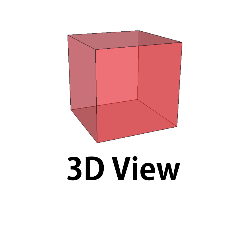
| 3D view
|
Pops up a window that shows a 3D view of the intensities of the currently selected mass peak. The sliders on the left hand side allow the user to slice through the data cuboid. | X | |||
| 3D overlay
|
X | ||||
| Reset ROI | Resets the shape of the red polygon in the left hand side figure. | X | X |