Dear user

A new version of simsMVA is out and it includes a number of new features. This will be a rather long list but we would like to highlight all major updates:

18 example datasets!

You can now find on the top menu 18 different example datasets of various different structures. This includes 4 examples of analytical techniques other than SIMS. This list of examples is as follows:

Imaging

• Particles: metal particles on an organic substrate.

• Blend: a cross-section of a polymer blend deposited onto a metal substrate (see publication).

• Adhesive 1 & 2: surface of an industrial adhesive with circular features.

• Droplet: surface of a topographical metal droplet.

Spectra

• Dicarboxylic acids: a set of spectra from standard dicarboxylic acids (see publication).

• Wood: spectra from wood samples together with standards for lignin and cellulose (see publication).

• Coffee: spectra of different types of coffee (see publication).

• Polypropylene: spectra of polypropylene-based composites with varying formulations.

Depth Profiling

• Metal multilayer: a dual-beam (Bi+ Cs+) depth profile of various different metallic layers.

• Organic/metal interface: a dual beam (Bi+ Ar_n+) depth profile of a hybrid interface.

3D Data

• Encapsulated polymer: a polymer “sphere” encapsulated by another polymer matrix.

• Copper grid: a copper grid on an aluminium substrate.

• Organic/metal interface: the 3D version of the depth profiling example.

Other Techniques

• Raman map: a Raman microscopy map of a droplet casted on SiO2.

• XPS profile: an XPS – C1s depth profile.

• PIXE map: a microbeam PIXE map of a cross-section.

• PIXE spectra: a set of various slightly different broad-beam PIXE spectra.

Save/Load project is now fully functional

Datasets can now be saved into .mat files and subsequently loaded in any other new tab of the same kind (Spectra, Profiles, Images or 3D).  No more stitching the same set of patches every time or waiting to load a long 3D dataset!

Completely revamped 3D visualisers 

Additionally to a series of bug fixes in the 3D data loader, the 3D visualiser and the 3D overlay tools were redesigned to allow more customisation (they are also now applicable to both the original data AND MVA results!).

The Z-correction tool has also been improved. The user can now pre-process the data and select whether to base the correction on a substrate or topographical feature

Convert 3D data into 2D and 1D

It is now possible to convert a 3D dataset into 2D (imaging) or 1D (depth profiling) data. The converted dataset will be loaded on a new tab, maintaining its “hyperspectral” aspect. This is an extremely useful tool that was developed out of need (no other software can do that).

Add peak labels in Imaging, Profiling and 3D modes

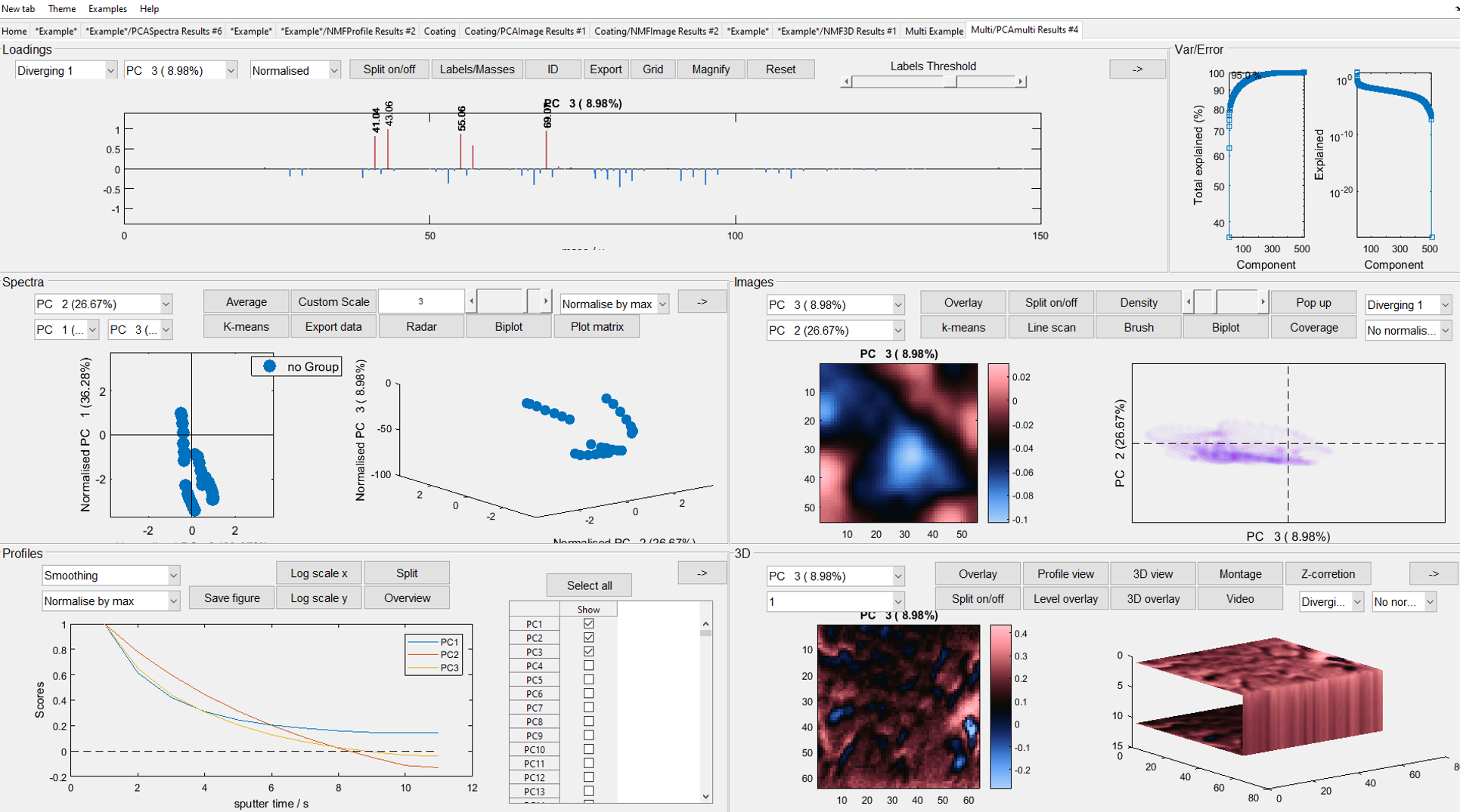
It had been long overdue, but it is finally possible to add peak labels in modes of analysis other than “Spectra”. A button has been added next to the variable selector in each mode.

Confidence intervals are now shown in Spectra PCA scores plots

And it is possible to change markers’ size!

Thank you very much for your support and feedback.

• See the previous updates here

• Download simsMVA